MS Excel

PREFACE:

Yes, ‘A dog is a man’s best friend’ and so is ‘Spreadsheet an accountant’s best friend’! And with Excel 2007, this friendship has only got stronger!! The new Avatar of Excel, i.e. the Excel 2007, by now is omnipresent and has finally cleared the doubts that were raised about its acceptability when it was launched about a three years back. Consequently this write-up is updated to include a few new tricks facilitated by the updated features in Excel 2007 and also show how to perform the old tricks with the new dog!!!

ABOUT THIS WRITE UP:

Learning Basic Excel: This write up is not meant to be a tutorial for beginners in MS Excel 2007. This write up presumes that the reader has working knowledge of Excel 2007. For beginners in MS Excel 2007, several free tutorials are available on the Internet. One such tutorial is at http://office.microsoft.com/en-us/excel-help/up-to-speed-with-excel-2007-RZ010062103.aspx

This write-up preliminary endeavors to accomplish the task of being a ready referencer of Excel for accountants. However the final objective of the write up is much beyond this. This write up is in four parts:

PART I - Self Learn Advanced Excel

Part II - TOP 51 Tips and Tricks

Part III - “Using Excel as Audit Tool”

PART IV - Links to Excel Resources

PART I - Self Learn Advanced Excel

The question most frequently asked to me has always been “How can I learn Advanced Excel?” The short answer is ”Use more of Excel”. You would then have many questions, which means so many opportunities to learn. To solve these questions and thereby self learn Excel, here is the route to follow:

The First place to look for help on Excel is in Excel itself. Press F1, type out your question and pat comes the reply. The help files are quite exhaustive and there are good chances that the solution to your query would be found on your desktop itself.
Come Home to Excel: There is a wealth of information on Excel at Microsoft Office Excel Home Page: http://office.microsoft.com/en-us/excel-help/office-excel-2007-product-overview-HA010165632.aspx?CTT=1
If this does not work, try searching Microsoft Excel 2007 support communities at http://answers.microsoft.com/en-us/office/forum/office_2007-excel?page=1 to find out if a similar question has already been asked and replied.
Search if an identical / similar issue has been addressed on Microsoft Knowledge database at http://search.support.microsoft.com/search/?adv=1
Search at web sites listed in Part IV – Links to Excel resources for tips and/or (free) addins to do what you want.
If you still cant find the solution, post a question to the Microsoft support community at the URL (web address) mentioned t point three above. (Click here to know the netiquettes of posting http://www.cpearson.com/excel/HintsAndTipsForNewsgroupUsers.aspx )

Part II – TOP 51 Tips and Tricks

Includes a collection of TOP 51 Tips and Tricks from the perspective of its utility to Chartered Accountants. The tips and tricks are in the form of solution to questions whose answer you always wanted to know. For questions that already have a solution posted on the Internet which can be accessed for free, I have simply provided the link to the solution to avoid re-inventing the wheel. Kindly note that while the questions are printed over here, for paucity of space, the solutions to them are on the CD.

How do I:

Entering and editing data, data validation

Create Shortcuts for commonly used words or phrases?
Quickly fill a series of Values?
Quickly fill Blank Cells in a list?
Suggest what is to be entered in a cell? (Cell Comment)
Change the User Name in the cell comment? Change the shape of the comment box?
Make Excel read out the contents of a worksheet?
Is there an alternative to Cell comment? (Data validation Input message)
Create Drop Down Lists?
Prevent duplicates while entering data?
Navigate to areas of worksheet efficiently / make formulas easier to read and understand?
Split Contents of Cells?
Combine Text from Multiple Cells?

Formatting, Key board Shortcuts, Copy paste

Format cells (e.g. highlight data) automatically based on a certain condition?
Automatically highlight maximum and minimum values in a list?
What are the Key board shortcuts to:

Go to the last used cell in a sheet?
Select cells from any cell to the last cell in the sheet's used range?
Move to the next / previous sheet?
Open new workbook? Insert new sheet?
Select entire row, Select entire column?
Insert current Date Insert current time?

Copy Paste only Values from one cell to another?
Convert Text to numbers?
Convert rows into columns?
Copy from Excel to Word?

Working with formulas and functions

My spreadsheet does not calculate at all, what’s wrong?
Toggle Between Relative and Absolute referencing?
Total if a condition is met?
See all formulas at the same time (formula view) in a worksheet?
Round off a number to the nearest 10 (to round off Total Income!!)?
Get the month of a date / day of a week? Quickly fill Blank Cells in a list?
Calculate the difference between two dates (e.g. calculate age in Excel)?
Count non blank cells? i.e. Cells that contain data?
Count blank cells? i.e. Cells that do not contain data?
Count cells that contain only numbers?
Monitor the value of a formula cell from any location?
Rank a number in a list?
Pick 20 random items (random sampling) from a list of 100 (population)?
Sort a list on more than three columns?

Applying auto filters, advanced filters, automatic subtotals

Quickly apply auto filter?
Filter for records containing text string / Use Wildcards in Criteria?
Remove Duplicates / Filter Unique Records?
Filter for more than one criterion?
Sum only visible rows in a filtered list?
Count visible rows in a filtered list?
Automatically summarize data by calculating subtotals?
Calculate subtotal within a subtotal?

Charts and Graphs in Excel:

Which is one of the Best resource on Excel Charting? (see also “Part IV Links to Excel Resources)

Emailing from Excel:

Where do I find all the information I need for emailing from Excel?

Financial functions

Calculate the effective annual interest rate where interest is compounded?
I am buying Government security that pays periodic interest. How do I calculate accrued interest on it?
Calculate the payment for a loan (for e.g. EMI) based on constant payments and constant interest rates?
Calculate interest rate that I am actually paying (and the lender is earning) on my home loan or car loan? (i.e. internal rate of return for a schedule of periodic cash flows)
Calculate internal rate of return for a schedule of cash flows that is not necessarily periodic (for e.g. in case of businesses where cash inflows and outflows are not periodic)?
Calculate Net Present value for a schedule of cash flows that is not necessarily periodic?
Calculate yield of a bond that pays periodic interest?

Macros And VBA:

I have heard a lot about Macros, but don’t know where to begin with. How do I start with Macros?

Part III – “Using Excel as Audit Tool”

Includes a series of four articles on “Using Excel as Audit Tool”. Of course MS Excel is best as a ‘means to an end’ for us. This powerful spreadsheet application package has earned the distinction of doubling up as an audit tool. Learning advanced Excel and then leveraging its power for our core competency, i.e. using Excel as a Computerised Assisted Audit Technique(CAAT) tool, is the objective of this series of articles. All the four articles are only in the CD. In all fairness I must mention that this series of four articles was first published in the BCA Journal in 2004-2005. However looking at its far reaching utility, it has been deemed fit to reproduce it over here. Click on the links below to access the articles.

Using Excel as an Audit tool – Part I

Using Excel as an Audit tool – Part II

Using Excel as an Audit tool – Part III

Using Excel as an Audit tool – Part IV

PART IV - Links to Excel Resources / Books on Excel

Includes links to the best resources on Excel. Learn Excel, explore VBA, pick up a tip, share a tip with others, download utilities for Excel and have fun. An almost exhaustive listing of the best links to Excel resources can be found at http://www.wittysparks.com/2009/04/17/list-of-useful-ms-excel-resource-sites/ and hence prudence suggest that no one should make any more. However a listing of Excel resources that I have found particularly useful are:

How to write spreadsheets: http://www.mang.canterbury.ac.nz/people/jfraffen/spreadsheets/index.html
Stephen Bullen's site contains great examples of various Excel programming and charting techniques: http://www.bmsltd.ie/
Excel information and tips at: http://www.mvps.org/dmcritchie/excel/excel.htm
A wealth of useful information: http://www.cpearson.com/excel.htm .
One of the best resources on Excel charting: http://peltiertech.com/

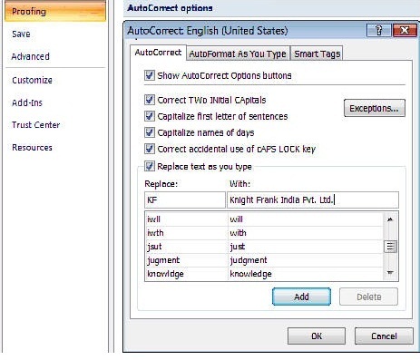
1. Create Shortcuts for commonly used words or phrases?

Use the AutoCorrect feature. It creates shortcuts for commonly used words or phrases.

Click Office Button à Excel Options à Proofing à AutoCorrect Options à AutoCorrect

On the [AutoCorrect] tab check the option ‘Replace Text As You Type’

Note that Excel Shares your AutoCorrect List with other Office Applications. AutoCorrect entries you created in Word will also work in Excel

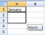
2. Quickly fill a series of values?

Use the AutoFill feature. It inserts a series of values or text items in a range of cells.

Drag the AutoFill handle (the small box at the lower right of the Active cell) to copy the cell or automatically complete the series

You can create your own list by adding a ‘Custom List’. To add a Custom List click <Office Button> à <Excel options> à <Popular> à <Edit Custom Lists..> and select the [Custom List tab]. In the [List entries] list box, type out your list entries separated by enter.

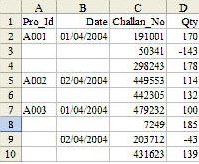
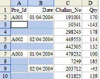
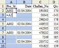
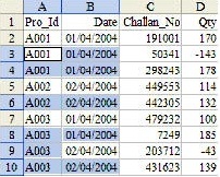
3. Quickly fill Blank Cells in a list?

Many times in a list, especially so when it is imported from a database, cells down below that have same headings or subheadings are left blank for the sake of easier readability. For eg. See the screenshot below

However this creates a difficulty when such lists are required to be sorted and/or subtotaled. To fill the cells down below with the subheadings of the cells above them, do the following:

Select the list
Click CTRL + G.
In the [Go To] dialogue box that appears, click the ‘Special’ button
In the [Special] dialogue box, select ‘blanks’. This will highlight only the blank cells in the list, with focus on the 1^st blank cell. See figure

In the 1^st blank cell, i.e. the cell with the focus, enter the formula =A2 (see figure) and press CTRL+ENTER.

As a result, the blank cells down below get filled up with the subheadings immediately above them. See figure

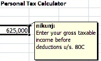
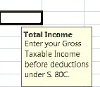
4. Suggest what is to be entered in a cell? (Cell Comment)

Cell Comment

Suggest the user as regards what is to be entered in the cell

Select the cell wherein you wish to see the message,
Right click and select <Insert Comment>.
Type the instruction in the comment box.

Note that the cell comment is displayed only when you move the cursor over the cell.

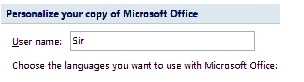
5. Change the User Name in the cell comment?

Click the Office button à Excel Options à Popular à Personalize your copy of Microsoft Office. A change here, changes the User name at the start of a comment.

Instead of showing the user name at the start of a comment, you can change to something generic, such as “Sir”.

To do this Click Office Button à Excel Options à Popular. Under the caption ‘Personalize your copy of Microsoft Office’, delete the existing User Name, and type a new entry. Click OK.

This change affects the User Name in all Microsoft Office programs.

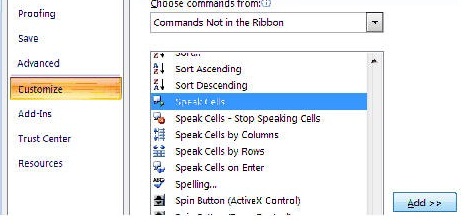
6. Make Excel read out the contents of a worksheet?

Use the Speak Cells feature. It reads the contents of a range / Reads data as entered

Get the Speak Cells button on the Quick Access Toolbar by clicking Office Button à Excel Option à Customize. In the [Choose commands from] list box, select [Commands Not in the Ribbon]. From the list of commands, select ‘Speak Cells’ and add it to the Quick Access Toolbar by clicking the <Add> button. Also add the ‘Speak Cells on Enter’ button.

To make Excel read out a range of cells, select the range first, and then click <Speak Cells> button.. To read the data as it is entered, click <Speak On Enter> button.

To adjust voice, Click My Computer à Control Panel à Speech. Select an option that you like in the [Text To Speech] tab.

7. Is there an alternative to Cell comment?

Yes, there is. It’s called Data validation Input message

Select the cell(s) in which you want to see the message. On the ribbon, click the <Data> tab then click <Data Validation>. Click the [Input Message] tab .Check the option 'Show input message when cell is selected'. Type your message heading text in the Title box. This text will appear in bold print at the top of the message. Type your message in the Input message box. Click OK.

Note that this message is displayed when you tab to the cell.

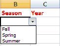
8. Create Drop Down Lists?

Haven’t you always wanted to create those lovely drop down list boxes to enter data in lists or forms for uniformity and standardisation? (See Figure)

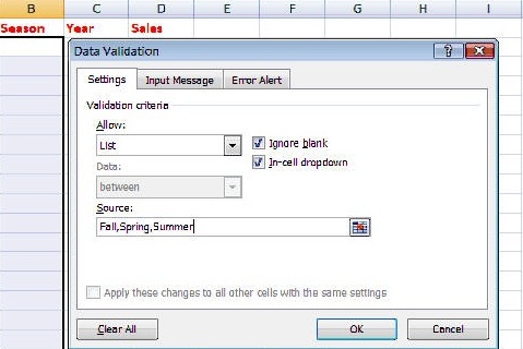
These are called data validation list boxes. Here’s how create them. In our example, Let us consider that you want the user to enter season in column B from a list of valid seasons. To create the List box for all cells in that column, select the entire column, except cell B1, and on the ribbon click <Data> à <Data Validation>

This will activate the [Data Validation] dialogue box. The [Settings] tab, prompts you for the validation criteria. In the first list box captioned Allow, select the option ‘List’. Now in the third list box captioned Source, type out the valid list separated by commas or refer to the range where valid seasons have been entered.

Note that you can also give a named range as the source of a valid list

In the Input message tab, you may enter a message like {Please Select A season from the List}. This may help the person who enters data as regards what is to be entered in that particular cell. In the Error Alert tab, you may enter a message like {Invalid Season, Only an item from the list is allowed!}. This message is flashed whenever the data entry person enters a season that is not one from the List. If you do not specify the Error Alert Message, Excel displays its standard Error Alert Message. That’s it! Click <OK>, and you are done. Now in every cell of column B, a list box appears as under. You may select the appropriate season, by simply clicking the drop down list box arrow. For Key Board addicts, who find it irritating to reach for the mouse every time the designation is to be entered, just go the cell in column D, and hit the [ALT + Down Arrow Key]

9. Prevent Duplicates while entering Data?

Use the Data Validation + Countif function. It Prevents the user from entering Duplicate data.

To do this:

1. Select a range of cells, for example, A2:A20.

2. On the Ribbon click <Data> à <Data Validation>

3. Select the [Settings] tab.

4. From the Allow dropdown list, select Custom.

5. In the Formula box, enter the following formula:

=COUNTIF($A$2:$A$20,A2)=1

6. Type an appropriate error message in the [Error Alert] Tab

10. Navigate to areas of worksheet efficiently / make formulas easier to read and understand?

Use the Named Range feature. It makes navigation efficient and makes formula easier to read and understand

To do it:

1. Select the cell(s) to be named

2. Click in the Name box, to the left of the formula bar

3. Type a one-word name for the list, e.g. ValidSeason

4. Press the Enter key

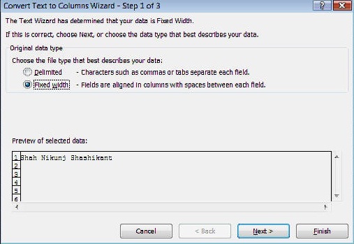
11. Split Contents of Cells?

Suppose you have entered the full name of a person in a particular cell and you now want to have Surname, First Name and Middle Name in three different cells. To do this, simply select the cell that contains the Full Name of the person, Click <Data> à <Text to Columns…>. This will activate the text to columns wizard (See Figure).

In step No 1 select the First radio button captioned <Delimited>, then click the <Next > button. In step No. 2, from the various types of Delimiters, select the check Box [Space]. You now see how the Full Name would be split into Surname, First Name and Middle Name. If you are fine with the display, click <Next>.

In step No. 3, amongst other things, you are asked to provide the cell address from where you would like the split text to appear. That’s it, on the main screen wizard of step Three click <Finish>. You now see the Full Name split into Surname, First Name and Middle Name in three different cells.

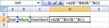
12. Combine Text from Multiple Cells?

Use the & (ampersand) operator

Lets you combine text from multiple cells

To combine text from multiple cells into one cell, use the & (ampersand) operator. Add a space between double quotes (“ “) to include a space in the combined text

13. Automatically format cells (e.g. change font color) based on a certain condition? Use the conditional Formatting. Conditional formatting allows you to set rules for cell formatting. If the rules (conditions) are met, then the formatting is applied. To do this:

1. Select the cells to be formatted

2. On the [Home] tab of the ribbon click [Conditional Formatting]

3. Leave the first drop-down box set to ‘Cell Value Is’

4. In the second drop-down box, choose one of the operators. Example, choose 'greater than'

5. In the text box, type a number or a cell reference. In this example, type the value you want to check – 499999.

6. Click the Format button

7. On the Patterns tab, select a colour for the conditional formatting -- blue, in this example.

You can also choose a Font format or a cell Border.

8. Click OK.

9. To add another conditional format, click the Add button.

10. Repeat steps 3 to 8, using the values and colours for the second conditional format.

11. Click OK, to return to the worksheet.

14. Automatically highlight maximum and minimum values in a list?

Conditional Formatting – Top/Bottom Rules

1. Select the Range.

2. On the [Home] tab click [Conditional Formatting] à Top/Bottom Rules à Top 10 items….

3. In the Top 10 items dialogue box specify the number of top items that you wish to highlight and the format for the same. Click <OK>

4. To highlight bottom values, on the [Home] tab click [Conditional Formatting] à Top/Bottom Rules à Bottom 10 items…

5. In the Bottom 10 items dialogue box specify the number of bottom items that you wish to highlight and the format for the same. Click <OK>

15. Which are amongst the most useful Keyboard Shortcuts?

Display or Hide the ribbon?

Press CTRL+ F1.

Go to the last used cell in a sheet?

Press CTRL + End.

Select cells from any cell to the last cell in the sheet's used range?

Press Shift + Ctrl + End to select cells from any cell to the last cell in the sheet's used range and Shift + Ctrl + Home to select cells from any cell to the first cell (A1) in the sheet's used range

Move to the next / previous sheet?

Press CTRL + Pg Up to go to next sheet and CTRL+ Pg Dwn to go to previous sheet.

Open new workbook?

Press Ctrl + N

Insert new sheet?

Press Shift + F11

Select entire row, Select entire column?

Press CTRL + Space Bar to select entire column and Shift + Space Bar to select entire row.

Insert current Date

Press CTRL ; to insert current date

Insert current time?

Press Shift + CTRL + ; to insert current time

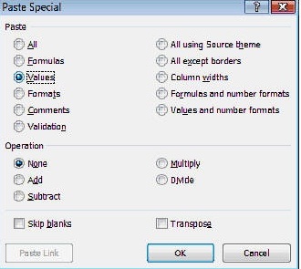
16. Copy Paste only Values from one cell to another?

Consider this example. Cell B3 contains the Formula =B1-B2 (see figure below).

This formula evaluates to 200. This ‘200’ is the value of Cell B3. To copy and paste this Value i.e. 200, to the adjoining cell C3, go to cell B3, hit [CTRL + C], or right your mouse and select <Copy> from the shortcut menu that pops up. Go to cell C3 and click <Edit> à <Paste Special>. A [Paste Special] dialogue box shall appear (See figure). . From the various options in the dialogue box, select the third option [Values] and click on <OK>. It’s done! Cell C3 now contains the value 200. In the same way you can copy and paste only the Formats (especially the conditional Formatting applied to a cell), Comments, Validation, etc, by selecting the appropriate button from the [Paste Special] dialogue box.

17. Convert Text to numbers?

In the Paste Special, select ‘Operation’ – ‘Multiply’. It converts text (that appears as numbers) to numbers. Follow the following steps:

In an empty cell, enter the number 1.
Select the cell, and copy
Select the range of text (appearing as numbers).
On the [Home] tab click [Paste] à <Paste Special>.
In the [Paste Special] dialogue that appears, under Operation, select Multiply.
Click OK.

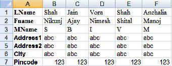
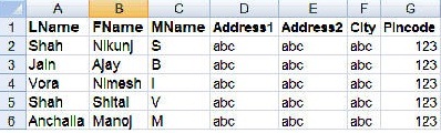
18. Convert rows into columns?

Well, consider this. You have created a sheet wherein headings like LName, FName, MName, Address1, Address2, etc, are arranged in rows while records appear as columns besides these headings (see Figure below).

Now, after entering around thirty to fourty records, you realise the obvious drawbacks of this layout and wish to rearrange the entire sheet by making the headings as columns and records below them as rows. This is what you can do. Select all cells, including the heading, and copy them. Open a fresh worksheet and select cell A1. Click <Edit> à <Paste Special…>. In the [Paste Special] dialogue box simply check the Transpose checkbox and click <OK>. That’s it. The sheet now looks as desired (see figure below).

19. Copy from Excel to Word?

Consider this. You have just finished typing out a lengthy report in Excel. At the very end, you realise that the report has hardly any calculations, and the formatting of the report would have been far better had the report been typed out in Word. So, you now wish to move only the entire text from the spreadsheet (Report) in Excel to Word and later on format it. This is what you can do. Select the entire report and copy it. Open a fresh document in Word. On the home tab, click <Paste Special…>. In the Paste Special dialogue Box, select the [Paste] radio button on the left hand side and form the [As:] list box select the third option [Unformatted Text]. Click <Ok>. That’s it. Now format the report the way you want!

20. My spreadsheet does not calculate at all, what’s wrong?

Calculation is set to Manual, alter this in Home à Excel Options à Formulas à Calculation options [Automatic]

21. Toggle Between Relative and Absolute referencing?

Press F4 when in Edit mode

When in Edit mode, select the reference you want to change and press F4

22. Calculate total if a condition is met?

Use the SUMIF() Function. It calculates total if a condition is met

1. Type an equal sign (=) to start the formula, Type: SUMIF(

2. Select the cells that contain the values to check for the criterion. In this example, cells C2:C211 will be checked

3. Type a comma, to separate the arguments

4. Type the criterion. In this example, you're checking for text, so type the word in double quotes: “Jackets”

5. Type a comma, to separate the arguments

6. Select the cells that contain the values to sum. In this example, cells E2:E211 will be summed

7. The completed formula is:

=SUMIF(C2:C211,“Jackets”,E2:E211)

23. See all formulas at the same time (formula view) in a worksheet?

The formula view is the normal method of showing formulas in Excel. To see all formulas instead of their calculated results, click the Office button à Excel Options à Advanced à Display Options for this worksheet à and check the option [Show formulas in cells instead of their calculated results]

Ctrl+₹ is the equivalent shortcut (toggle on/off) -- accent grave to left of the 1,2,3 on the top row

24. Round off a number to the nearest 10

Use the Round () function to do this. For eg. Round(A1,-1) rounds the number in cell A1 to nearest 10s

25. Get the month of a date / day of a week?

MONTH() function/WEEKDAY() function

Use the MONTH() function to get the month from a date. To get the day of the week, use the WEEKDAY() function

Note: To display the day of the week spelled out, set the number format of the cell dddd

26. Calculate the difference between two dates (e.g. calculate age in Excel)?

Use the Datediff function to do this. Where date of birth is entered in Cell C2 and today’s date in cell D2, the following formula will calculate the age in completed years, months and days: =DATEDIF(C2,D2,"y") & " years, " & DATEDIF(C2,D2,"ym") & " months, " &DATEDIF(C2,D2,"md") & " days, "

27. Count non blank cells? i.e. Cells that contain data

Use the =COUNTA() FUNCTION

28. Count blank cells? i.e. Cells that do not contain data

Use the =COUNTBLANK() function

29. Count cells that contain only numbers?

Use the =COUNT() function

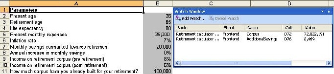
30. Monitor the value of a formula cell from any location?

Use the Watch Window feature

If you have a spreadsheet model you may find it helpful to monitor the values in a few key cells as you change few input cells. To watch a cell, select the cell. On the Formulas tab of the ribbon click Watch Window. Excel displays a floating window titled [Watch Window]. Click <Add Watch> à Add. See figure

32. Pick 20 random items (random sampling) from a list of 100 (population)?

Use RAND() formula to do this. Say your population is in column A from A1:A100. In B1:B100 enter formula =RAND(). Sort the list by B column; top 20 rows is your selection. Press F9 for new numbers in column B and repeat for a new selection.

33. Sort a list on more than three columns? (For Excel 2002/03/XP)

Use sort Ascending or sort Descending buttons on the standard toolbar

Start with the “least significant” sort and end with the “most significant” sort. Example to sort a sales file by Year, Season, Type and State, first sort by State, then by Type, then by Season and then by Year.

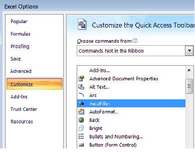
34. Quickly apply auto filter?

Add AutoFilter icon to quick access toolbar

1. Click Microsoft Office button à <Excel Options>.

2. In the <Excel Options> dialog box, click ‘Customize’.

3. In the Choose commands from list box, select ‘Commands Not in the Ribbon’.

4. Select the AutoFilter icon (Funnel shaped)) from the list below and add it to the Quick Access toolbar.

5. Click OK.

35. Filter for records containing text string / Use Wildcards in Criteria?

Use wildcard characters to filter for a text string in a cell.

The * wildcard

The asterisk (*) wildcard character represents any number of characters in that position, including zero characters. In this example, any customer whose name contains "Mall" will pass through the filter.

The ? wildcard

The question mark (?) wildcard character represents one characters in that position. In this example

any 4-letter product that begins with ‘c’, and ends with ‘ke’ (eg. Coke, Cake) will pass through the filter.

The ~ wildcard

The tilde (~) wildcard character lets you search for characters that are used as wildcards. In this example, only the product named Good*Eats, will pass through the filter.

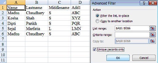
36. Remove duplicates / Filter Unique Records?

You can use an Advanced Filter to extract a list of unique items in the list. To do this, click on <Data> à filter à <Advance filter>. In the [Advanced Filter] dialogue box that opens, check out the ‘Unique records only’ option (See figure below). That’s it. You are done.

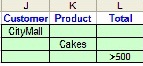
37. Filter for more than one criterion?

Use ‘Criteria range:’ in the [Advanced Filter] dialogue box to filter a list that meets a given criteria. You can use more than one criteria to filter a list as well.

To filter a list for records that meet ALL the criteria, write all conditions in one row. This shall filter the list for records that meet all the conditions. For example writing the criteria in this way shall filter the list for records where -

Customer = CityMall AND Product = Cakes AND Total = greater than 500.

To filter a list for records that meet ANY of the criteria, write conditions in different rows. This shall filter the list for records that meet any of the conditions. For example writing the criteria in this way shall filter the list for records where -

Customer = CityMall OR Product = Cakes OR Total = greater than 500.

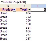
38. Sum only visible rows in a filtered list.

To sum only visible rows which contain data, you can use the Subtotal function in a formula in the same row as your headings. For example,

to sum the visible entries in column D which contain numbers, you could use this formula: =SUBTOTAL(9, D:D) . The number ‘9’ in the first part of the formula, tells Excel to ‘Sum’ the numbers in column D.

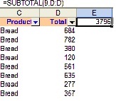
39. Count visible rows in a filtered list?

Similarly, to count the visible rows in a filtered list, use the Subtotal formula with number ‘2’ in the first part of the formula. For example,

The formula used in the above screenshot counts the number of visible rows in column D.

40. Automatically summarize data by calculating subtotals?

Use the Subtotal feature to do this.

To insert subtotals into a list, first sort the list.

Click a cell in the sorted list, and then click [Data] à[Subtotal].

41. Calculate subtotal within a subtotal?

Uncheck ‘Replace Current Subtotals’ in the [Subtotal] dialogue box

1. First sort the list.

2. Click a cell in the sorted list, and then click [Data] à[Subtotal].

3. Repeate step No. 2, but Uncheck ‘Replace Current Subtotals’ in the [Subtotal] dialogue box

42. Which is one of the Best resources on Excel Charting? (see also “Part IV Links to Excel Resources)

Check out http://peltiertech.com/. It is one of the best resources on Excel charting

43. Where do I find all the information I need for emailing from Excel?

Check out Ron de Bruin Microsoft MVP – Excel site at http://www.rondebruin.nl/ Here you can find all the information you may ever need for emailing from Excel.

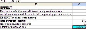
44. Calculate the effective annual interest rate where interest is compounded?

Use EFFECT(nominal_rate,npery) function to calculate the effective annual interest rate, given the nominal annual interest rate and the number of compounding periods per year.

Syntax

EFFECT(nominal_rate,npery)

Nominal_rate is the nominal interest rate.

Npery is the number of compounding periods per year. e.g. 2 if compounded semi-annually, 4 if compounded quaterly.

For e.g. where the nominal interest rate is 5.25% p.a. and the compounding is quaterly, the effective interest rate works out to be 5.3543%. See figure.

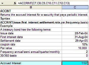
45. I am buying Government security that pays periodic interest. How do I calculate accrued interest on it?

Use the AccruedInt() function to calculate accrued interest on a security that pays periodic payment.

Syntax

ACCRINT(issue,first_interest,settlement,rate,par,frequency,basis)

Issue is the security's issue date.

First_interest is the security's first interest date.

Settlement is the security's settlement date. The security settlement date is the date after the issue date when the security is traded to the buyer.

Rate is the security's annual coupon rate.

Par is the security's par value. If you omit par, ACCRINT uses $1,000.

Frequency is the number of coupon payments per year. For annual payments, frequency = 1; for semiannual, frequency = 2; for quarterly, frequency = 4.

Basis is the type of day count basis to use.

For e.g. see figure

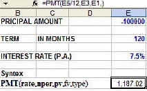
46. Calculate the payment for a loan (for e.g. EMI) based on constant payments and constant interest rates?

Use the PMT() function to Calculate the payment for a loan (for e.g. EMI) based on constant payments and constant interest rates.

Syntax

PMT(rate,nper,pv,fv,type)

Rate is the interest rate for the loan.

Nper is the total number of payments for the loan.

Pv is the present value, or the total amount that a series of future payments is worth now; also known as the principal.

Fv is the future value, or a cash balance you want to attain after the last payment is made. If fv is omitted, it is assumed to be 0 (zero), that is, the future value of a loan is 0.

Type is the number 0 (zero) or 1 and indicates when payments are due.

For e.g. see figure

Note: you can also use PMT function to calculate payments to annuities other than bank loans. For e.g. you can calculate the amount required to be saved per month to accumulate a sum of amount at the end of a given period where your savings earn interest as well.

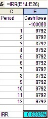
47. Calculate interest rate that I am actually paying (and the lender is earning) on my home loan or car loan? (i.e. internal rate of return for a schedule of periodic cash flows)

Use the IRR function to calculate internal rate of return for a schedule of periodic cash flows. The cash flows do not have to be even, as they would be for an annuity. However, the cash flows must occur at regular intervals, such as monthly or annually. The internal rate of return is the interest rate received for an investment consisting of payments (negative values) and income (positive values) that occur at regular periods.

For e.g. see figure

48. Calculate internal rate of return for a schedule of cash flows that is not necessarily periodic (for e.g. in case of businesses where cash inflows and outflows are not periodic)?

Use the XIRR() function. It returns the internal rate of return for a schedule of cash flows that is not necessarily periodic. To calculate the internal rate of return for a series of periodic cash flows, use the IRR function.

Syntax

XIRR(values,dates,guess)

Values is a series of cash flows that corresponds to a schedule of payments in dates. The first payment is optional and corresponds to a cost or payment that occurs at the beginning of the investment. If the first value is a cost or payment, it must be a negative value. All succeeding payments are discounted based on a 365-day year.

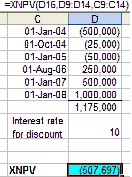
49. Calculate Net Present value for a schedule of cash flows that is not necessarily periodic?

Use the XNPV() function to Calculate Net Present value for a schedule of cash flows that is not necessarily periodic.

Syntax

XNPV(rate,values,dates)

Rate is the discount rate to apply to the cash flows.

Dates is a schedule of payment dates that corresponds to the cash flow payments. The first payment date indicates the beginning of the schedule of payments. All other dates must be later than this date, but they may occur in any order.

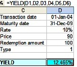
50. Calculate yield of a bond that pays periodic interest?

Use the YEILD() function to calculate yield of a security that pays periodic interest.

Syntax

YIELD(settlement,maturity,rate,pr,redemption,frequency,basis)

Important Dates should be entered by using the DATE function, or as results of other formulas or functions. For example, use DATE(2008,5,23) for the 23rd day of May, 2008.

Settlement is the security's settlement date. The security settlement date is the date after the issue date when the security is traded to the buyer.

Maturity is the security's maturity date. The maturity date is the date when the security expires.

Rate is the security's annual coupon rate.

Pr is the security's price per $100 face value.

Redemption is the security's redemption value per $100 face value.

Frequency is the number of coupon payments per year. For annual payments, frequency=1; for semiannual, frequency = 2; for quarterly, frequency = 4.

For e.g. see figure

51. I have heard a lot about Macros, but don’t know where to begin with. How do I start with Macros?

The best place to start with Macros and VBA is to go through Microsoft’s tutorial archived at http://web.archive.org/web/20031204013634/support.microsoft.com/default.aspx?scid=/support/excel/content/vba101/default.asp . Also check out this link for explanation on macros, VBA and User defined Functions:http://www.mvps.org/dmcritchie/excel/getstarted.htm